Performance

Showcase panel 08: circles and friends: hundreds of shapes in four calls.

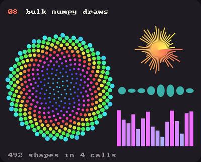
Showcase panel 08: circles and friends: hundreds of shapes in four calls.
Try it live: run uv run python examples/showcase.py, then hover panel 08, or see the showcase.

Kiln can draw hundreds of thousands of shapes in a frame. This page explains why, then shows how to ask for that speed.

Why Kiln is fast

Three ideas do all the work:

Batched records. circle does not touch the GPU. It appends one small record (20 numbers: a transform, the shape, a colour) to a list and returns.
One upload per frame. At the end of the frame every record goes to the GPU in a single transfer, and the shapes are drawn in a handful of GPU calls, not one per shape.
SDF shapes on the GPU. Each record is a signed distance function: the GPU shades a small quad per shape and works out, for each pixel, how far it is from the outline. That is why edges are crisp and anti-aliased at any size and why a circle costs a record, not a polygon of triangles.

So the cost of a frame is mostly the time Python spends writing records. Each circle call is cheap, but it is still a Python call. That is the part the bulk functions remove.

Why these choices

Each idea above was picked over an alternative, the backend on a benchmark and the rest on the cost of a Python call. Knowing why tells you where Kiln is quick and where it isn’t.

OpenGL 4.1 through zengl, not Metal or WebGPU. From Python, what limits a frame is the cost of each GPU call, not the GPU. On the M3 Pro development machine, 5,000 draw calls a frame cost 3.4–5.1 ms with zengl, 7.4–10.7 ms with moderngl, 4.7–9.9 ms with Metal driven directly from Python and 11.1–16.4 ms with wgpu-py; streaming a million vertices was a tie. Metal would have cost a second shader language and bought no per-call speed from Python. OpenGL 4.1 is the newest version macOS offers, so GLSL is what you write. The GL code stays in a few modules under kiln.graphics, so the backend can be swapped later without touching your sketches.
Records, not GPU calls. One draw call per shape would put the per-call cost above on every circle. Applying the transform and appending a record costs about 0.65 µs in plain Python, so 10,000 calls fit in under 7 ms. The records are uploaded once, at the end of the frame (plus an extra flush if, say, you load or release a texture mid-frame), and never rewritten while an earlier draw still reads them, which would stall the GPU.
Signed distance fields, not triangles. Cutting each shape into triangles on the CPU costs far more Python: in the README’s benchmark a five-vertex polygon costs about 13 µs, a circle about 0.7 µs. A distance field costs one record whatever the size, and the GPU anti-aliases the edge for free. The cost moves to the pixels: a shape costs what it covers, which is why large ellipses are the dearest shape.
The transform rides in the record. with transform(), translate and rotate change no GPU state, so they never split the batch.
Runs, in your order. Records are drawn in the order you made them. A run of the same kind of draw is one GPU call, and a new run starts when the blend mode, the texture, the shader (or one of its uniforms) or the target Fbo changes, or when the kind changes (an SDF shape against a custom shape or a picture, say). A typical frame is a handful of GPU calls.
Nothing is compiled per frame. Each shader program is compiled once. The pipeline for a combination of kind, blend, target, texture and shader is built the first time it is drawn and reused after that.
Custom shapes are the exception. Anything with shape() makes (curves, beziers, holes) has no distance field, so it is cut into triangles on the CPU: earcut for fills, a mitred strip for outlines. That is Kiln’s slow path. In the README’s benchmark, 1,000 five-vertex polygons take 12.7 ms where 10,000 circles take 6.8 ms, and a self-crossing fill grows roughly with the square of its vertex count (about 11 ms at 300 vertices, 30–40 ms at 600).
numpy for bulk, the GPU for more. The bulk calls build every record with a few numpy operations, at 10 to 15 ns a shape. Past that, the work leaves Python altogether: instancing sends per-copy data once, and GPGPU simulations never come back to the CPU. Kiln needs only zengl, glfw, numpy, earcut and Pillow to run, with no compiler step.

What this costs: a loop of single calls is bound by Python, so a framework compiled to native code will run it faster, and self-crossing filled shapes are slow today. Kiln is built to be quickest on many simple shapes, numpy arrays and work the GPU does by itself.

Immediate versus bulk

circles, ellipses, rects and lines take numpy arrays and write all the records at once. They draw exactly what a loop of single calls would, in the same order, with the same fill, line width, blend mode, rect mode and transform.

import numpy as np
import kiln

rng = np.random.default_rng(1)
xy = rng.uniform(0, (400, 300), (600, 2))      # centres, shape (n, 2)
radius = rng.uniform(3, 14, 600)               # one radius per circle, shape (n,)
colors = rng.uniform(80, 255, (600, 3))        # one colour per circle, 0-255

def draw():
    kiln.background(14, 16, 28)
    kiln.circles(xy, radius, colors)

show(draw)

The arguments are plain arrays:

xy is (n, 2). lines(p1, p2) takes two (n, 2) arrays instead.
radius (or size) is one number for every shape, or an array of (n,). size also accepts (n, 2) for a width and height per shape, and [[w, h]] for one width and height for all of them (a bare (w, h) is refused, since with two shapes it could mean one size each).
color is None (the current colour), one colour, or an (n, 3) or (n, 4) array of 0 to 255 values. Fill, line width and the transform come from the current style, as with the single calls.

A wrongly shaped array raises a ValueError that says what was expected.

How much faster?

The cell below measures it on this machine: the time Python spends inside the drawing calls (“record build”), and the whole frame including the GPU and the read-back (“full frame”), as the median of several frames. These numbers are indicative: they move with what else the computer is doing.

import datetime, os, statistics, time
import numpy as np
import kiln
from IPython.display import Markdown
from kiln.testing import render_frames

class Timed(kiln.App):
    def __init__(self, fn):
        self.fn, self.cpu = fn, []

    def draw(self):
        kiln.background(10, 10, 20)
        t = time.perf_counter()
        self.fn()
        self.cpu.append(time.perf_counter() - t)

def measure(fn, frames=7):
    """Median (record build ms, full frame ms), ignoring the warm-up frame."""
    app, stamps = Timed(fn), []
    render_frames(app, frames=frames, size=(800, 600),
                  on_frame=lambda _: stamps.append(time.perf_counter()))
    return (statistics.median(app.cpu[1:]) * 1e3,
            statistics.median(np.diff(stamps)[1:]) * 1e3)

rng = np.random.default_rng(0)
rows = []
for n in (10_000, 100_000, 1_000_000):
    xy = rng.uniform(0, (800, 600), (n, 2))
    r = rng.uniform(1, 4, n)
    if n == 10_000:
        pts, rs = xy.tolist(), r.tolist()
        def immediate():
            kiln.fill(255, 160, 60)
            for (x, y), rr in zip(pts, rs):
                kiln.circle(x, y, rr)
        build, full = measure(immediate)
        rows.append(f"| `circle` x {n:,} | {build:.1f} | {full:.1f} |")
    build, full = measure(lambda: kiln.circles(xy, r, (255, 160, 60)))
    rows.append(f"| `circles`, {n:,} | {build:.1f} | {full:.1f} |")

load = os.getloadavg()[0]
Markdown("| 800x600 frame | record build (ms) | full frame (ms) |\n|---|---:|---:|\n" + "\n".join(rows)
         + f"\n\n*Measured {datetime.date.today()} at a load average of {load:.1f}"
         f" on {os.cpu_count()} cores: a busy machine makes these times longer.*")

800x600 frame	record build (ms)	full frame (ms)
`circle` x 10,000	6.5	8.8
`circles`, 10,000	0.1	1.3
`circles`, 100,000	0.8	4.1
`circles`, 1,000,000	9.2	22.4

Measured 2026-10-13 at a load average of 4.9 on 12 cores: a busy machine makes these times longer.

Two things stand out. Per shape, the bulk call writes a record in tens of nanoseconds (10 to 15 ns on a quiet machine, per the benchmark in the README), where a circle call costs a good fraction of a microsecond (about 0.65 µs when quiet), so building 10,000 records is dozens of times faster whatever the load. And the full frame then becomes GPU and upload work, which grows roughly linearly with the shape count, not with Python call overhead. Every figure above is higher than on a quiet machine, because the render shared the computer with other jobs.

Tips

Avoid per-frame Python loops over shapes. Compute positions, sizes and colours with numpy (kiln.noise takes arrays too) and hand the arrays over.
Prefer bulk calls beyond about 10,000 shapes. Below a few hundred shapes the single calls are just as good and read better.
Keep the arrays between frames and update them in place (p += v) instead of rebuilding lists.
Draw one shape thousands of times with instancing. When every copy is the same mesh with different data (position, colour, angle), a Vbo and draw(instances=) send the data once and draw all of them in one call: 4,096 fish rewritten every frame take about half a millisecond.
Move the simulation to the GPU when the particles outnumber what numpy can update in a frame: GPGPU particles steps a quarter of a million of them in a float Fbo, with no Python in the loop.
Keep static geometry on the GPU. A Vbo is uploaded once and drawn again for free, where a Mesh is sent again at every draw.
Large ellipses are the costly shape: their distance function is the most expensive, and big shapes shade more pixels. Circles, rectangles and lines are the cheapest.

A stress scene

examples/stress.py (“Supernova”) is the benchmark you can watch. It runs five layers at once, each aimed at a different cost in the pipeline:

galaxy: up to millions of particles, numpy physics and one circles call;
plexus: about 900 noise-driven nodes, every pair closer than 80 points linked, thousands of segments in one lines call;
rain: thousands of bitmap glyphs, one text call per column;
fractal: a Pythagoras tree of thousands of immediate-mode with transform(), rotate, scale and rounded rect calls;
rose: a self-crossing rose curve, re-tessellated every frame under a NONZERO winding rule, the costliest fill there is.

The panel at the top left times each layer’s Python record-building and plots the frame time. The video below is the scene with the galaxy doubled twice, to 400,000 particles (press + twice). The ms column is real, measured while this page was rendered, on a computer that was busy with other jobs (a quiet one is several times faster). The big “fps” and “frame” figures are not: the docs render this video on a pinned clock of 30 fps, so those two always read 30.0 and 33.3 ms. Run the example to see yours.

supernova: 400,000 particles at exit, 30.0 fps

Keys. 1 to 5 toggle a layer, + and - double or halve the particles, a auto-ramps the galaxy until the frame rate gives way (and hovers near the largest count that keeps roughly 51 to 57 fps), [ and ] change the rose’s vertices, , and . the fractal depth, t toggles the trails, h the panel, space pauses, esc quits. The mouse: the left button pulls the galaxy in, the right button blows it apart, and the scroll wheel changes the rose’s petal count. The rose fill costs about n squared in its vertex count: at the 3,000 maximum, expect a fraction of a second per frame.

Run it with uv run python examples/stress.py.

Try this: 100,000 particles in a noise flow field

Every particle follows the direction of a 3D noise field, and all 100,000 are moved, coloured and drawn with a few array operations per frame. No loops over particles.

import math
import numpy as np
import kiln

N = 100_000

class FlowField(kiln.App):
    def setup(self):
        rng = np.random.default_rng(5)
        self.p = rng.uniform(0, (400, 300), (N, 2))
        self.t = 0.0

    def update(self):
        self.t += 0.004
        a = kiln.noise(self.p[:, 0] * 0.005, self.p[:, 1] * 0.005, self.t) * math.tau * 2
        self.a = a
        self.p += np.column_stack([np.cos(a), np.sin(a)]) * 1.2
        self.p %= (400, 300)

    def draw(self):
        kiln.background(8, 10, 22)
        kiln.blend(kiln.Blend.ADD)
        hue = self.a / (math.tau * 2)
        colors = np.column_stack([60 + 195 * hue, 90 + 80 * (1 - hue), 255 - 150 * hue, np.full(N, 70)])
        kiln.circles(self.p, 0.9, colors)
        kiln.blend(kiln.Blend.ALPHA)

show_video(FlowField(), frames=45, fps=30, width=300)

Change 0.005 for tighter or broader currents, the 1.2 for speed, and the alpha 70 for how quickly the glow builds up where the particles bunch together.